Understanding Sparse Autoencoders
16 min read
·…
tl;dr:Learning the principles of SAE.
Lately, most of my time has gone into vibing on my meeting transcription tool Brevia. If I were updating the blog more systematically, I would probably be writing development logs instead. But while testing the tool, I listened to Google DeepMind’s latest podcast on interpretability in large language models, featuring Neil Nanda, who leads their interpretability team.
Throughout the conversation, they discussed why interpretability matters, how it might be achieved, and what it can be used for. In one segment, they mentioned Sparse Autoencoders (SAEs) and described them as one of the more fashionable techniques right now for learning activations that are irrelevant most of the time, but crucial at the right moment.
That caught my attention. Earlier, while studying generative recommendation systems, I had run into information-compression methods such as RQ-VAE, which compress high-dimensional inputs into sparse semantic codes. I wondered whether the two might play somewhat similar roles, so I spent some time reading up on SAEs.
Relevant content from the podcast
I’ll start with the notes I took from the podcast itself:
Sparse Autoencoders (SAE)
Main Discussion:
-
SAE has a goal similar to that of probes: telling us what a model is “thinking.” But unlike probes, it does not require us to specify the concepts in advance. Instead, it tries to automatically discover the concepts a model may be representing. A useful analogy is brain imaging: the raw signal looks like a mess, but if you stare at it long enough, patterns begin to emerge. One “ripple” lights up when a person sees light, another when they speak, and another when they listen. SAE is a machine learning technique for discovering those “ripples” that are absent most of the time but highly important when they do appear, because those ripples may correspond to real concepts. In principle, you can end up with tens of thousands or even millions of discovered concepts. What makes SAE exciting is that it can surface things you would never have thought to look for.
-
Example for understanding hallucinations (from a paper Neil supervised): SAE can pick up concepts like “I recognize this entity” and “I do not recognize this entity.” If you give the model the Beatles song “Yellow Submarine,” it recognizes it; if you give it “Turbo Y Submarine” or “turquoise submarine,” it does not. When it recognizes something, it answers questions; when it does not, it says, “I don’t know.” You can even edit these concepts. If you make the model act as if it does not recognize Yellow Submarine, it stops answering; if you make it act as if it does recognize turquoise submarine, it starts trying to answer and makes things up. That gives us a useful signal for detecting hallucinations. Later papers pushed further on this “hallucination probe” direction, though the method may still be too imprecise for consumer-facing systems. It is still a very promising line of research.
-
Prism analogy: a model is like white light. White light contains many wavelengths, many colors, but to us it still looks white. A model may be “thinking” about hundreds of concepts at once, such as “am I near the end of a sentence,” “is the next word a noun or a verb,” or “what emotion does the character I’m simulating have.” We only see a vector of numbers because all of those concepts are mixed together, but in principle there are ways to separate them.
Limitations:
The concepts discovered automatically by SAE are not always correct. Neil treats this as a trade-off: if you know exactly what you want and have good data, training a probe is usually the better option. But if you do not have good data, or you do not even know what to look for yet, then a tool like SAE, which is “not entirely reliable but still very useful,” can be a good first step. Sometimes it is the only step you need, and often it tells you what to look for next so that you can go collect better data. One practical issue is that some concepts simply fail to show up. For example, if the corpus used to train the SAE does not contain enough chat data, it may miss important concepts such as “refusing harmful requests.”
Sparse Regularization
The earliest roots of SAE go back to the 1980s. In a 1996 Nature paper from computational neuroscience, researchers built a model for reconstructing images and added a penalty term, similar to regularization, that encouraged the model to reconstruct an image using as few active neurons as possible. The goal was to understand why biological neurons respond to certain regions of visual input.
Computational neuroscience was much further ahead than I had imagined. By 1996, people were already formalizing biological neural responses numerically and had a fairly clear grasp of receptive fields. I should spend more time on that topic later.
Sparse Autoencoders
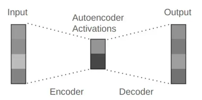
After 2000, autoencoders became popular, with reconstruction loss as the core training objective. SAEs appeared soon afterward by adding a sparsity constraint, essentially a regularization term, on top of reconstruction loss. At the time, these methods were mainly used for representation learning and dimensionality reduction, with an emphasis on learning features that were more meaningful and more localized.
After reading a few references and talking with GPT, the rough explanation that made sense to me starts from the context of that era. Back then, machine learning relied heavily on handcrafted features, whether engineered feature crosses in recommendation systems or SIFT/HOG in computer vision. So a lot of research was aimed at learning features automatically. Autoencoders were one route. The idea was that if you only optimize for accurate image reconstruction, the model may learn representations that are not especially useful. Adding sparsity forces the model to rely on only a small number of weighted activations, making it more likely to capture the important information.
A common workflow at the time was to train an SAE on a large set of images in an unsupervised way, let it learn image representations, and then feed labeled images through the trained SAE to obtain representation vectors, which were then passed to an SVM for classification.
Why Not Directly Train SVM with 10,000 Images?
GPT: This is precisely the key question of that era. Traditional SVM, if directly fed raw pixels, those raw pixels aren’t necessarily good representations for classification. People used to manually design HOG and SIFT, while SAE used unsupervised learning of intermediate representations to solve this problem.
I then asked whether this was similar to the CNN-plus-embedding pattern. GPT’s answer was that they are related, but not the same: SAE is closer to learning embeddings in a self-supervised way.
Interpretability and Philosophy
Deep learning kept racing forward after 2010, but by the 2020s it had run into the problem of interpretability. A central issue is that a single neuron may respond to multiple features. It might fire for an animal name and also for some completely unrelated technical term. This is known as polysemanticity, and one theoretical explanation for it is superposition: the model needs to represent far more latent features than it has neurons available.
In a Transformer, many features can be represented within a limited -dimensional space by occupying different directions in that space. In other words, one feature is typically distributed across multiple neurons.
If a model has only a 4096-dimensional representational space, but needs to encode 100,000 potential semantic features, it will reuse those dimensions in different weighted combinations to represent different features:
A single feature is therefore represented across many neuronal dimensions. For example, Python might correspond to , while DNA might correspond to .
Because these are weighted combinations, different neurons contribute differently. For any given feature, perhaps only a few coordinates are strongly non-zero. What we observe from the outside is that the same neuron participates in representing multiple features, which is exactly polysemanticity. SAE tries to disentangle that 4096-dimensional activation vector into a sparser feature space.
I tried to understand this through the lens of embeddings:
“Isn’t this basically what embeddings already do? A feature is a high-dimensional vector, there are too many features for one-hot representations to work, so we use embeddings. Embeddings are hard to interpret, so then SAE comes in?”
GPT explained it like this:
“Your intuition is very close, but there’s a key point to correct:
Embedding and superposition are indeed mathematically similar in form, but ‘too many tokens so can’t one-hot → embedding’ and ‘too many features so can’t have one neuron per feature → superposition’ are problems at two different levels.”
They form a very nice analogy. Embedding solves the problem of having too many tokens by assigning low-dimensional dense representations to a large number of discrete objects.
Superposition addresses a different issue: there are too many internal semantic features to represent cleanly. If you tried to give each feature its own one-hot-style neuron, you would run out of capacity, so many features end up packed into the same low-dimensional dense representation.
The key distinction is that embedding is “object -> vector,” whereas superposition is “multiple features -> the same vector.” A token embedding is a lookup from one token to one vector. A hidden state, by contrast, is a superposition of multiple active features.
Ideally, suppose the vector for French is . We do not know what each coordinate means, but we hope SAE can map it into a new coordinate system like , where only a small number of features are active.
In the idealized picture, that new vector would be close to one-hot, with each dimension corresponding to one interpretable feature. For example, dimension 1837 might mean city and dimension 2000 might mean Europe, and a small number of such dimensions would combine to form the representation of French.
So embedding packs many things into a low-dimensional distributed space, while SAE tries to do the reverse: unfold that distributed space back into a sparse feature space.
My next question was: “If we cannot fully recover a one-hot representation, then even after we move into a sparse space, humans still do not really understand it, right?”
GPT:
That is exactly the most important “last mile” problem in SAE interpretability. We may know that feature 1837 fired with value 2.7, but what is feature 1837 actually supposed to mean?
What researchers actually do is run LLM activations through an SAE to produce sparse features, and then inspect which inputs activate each feature most strongly. That is how they attach an interpretation to it.
For example, after training an SAE, suppose researchers discover feature #1837. They feed a large amount of text through the model and look for the inputs that maximize the activation of that feature:
Suppose the strongest activations come from examples like:
“He moved to San Francisco in 2019.”
“The population of New York City increased…”
“She currently lives in Tokyo.”
“Paris is the capital of France.”
Then a human, or perhaps another LLM, might summarize that pattern as: “Feature 1837 is roughly about city names, or cities more broadly.”
And if you keep pushing, you run into SAE’s biggest problem. Suppose feature #1837 activates for Paris, Tokyo, London, and Madrid. We may say it means city, but perhaps it really means place names, or major cities, or capital-related text, or even some concept that natural language cannot describe well at all. So the features produced by SAE cannot be said to be perfectly human-interpretable in any strict sense.
At that point, the topic became more interesting to me. It occurred to me that linguistics and cross-cultural studies probably have many related ideas here about how abstract concepts can be described in a more formal way.
There is a field called corpus linguistics. If researchers do not know the exact meaning or usage pattern of a word, they can study a large body of real language data. For example, if you wanted to study what home means across cultures, you could gather a large corpus, look at the contexts in which home appears, and infer an approximate bundle of meanings: residence, family, belonging, hometown, and a sense of safety.
“You shall know a word by the company it keeps.”
That line is a famous idea in linguistics. And later, major NLP ideas such as Word2Vec and embeddings grew out of that same intuition.
It is interesting to see different disciplines meet around the same core idea. Once machine learning reaches interpretability, the discussion quickly stops being a purely technical one and starts touching linguistics, cognitive science, and even philosophy.
LLM and SAE
In 2023, the paper Sparse Autoencoders Find Highly Interpretable Features in Language Models connected SAE to modern LLMs. The core idea was to use SAEs to reconstruct internal activations in language models so as to recover more interpretable features.
Anthropic also explained this direction in an October 2023 blog post. Their idea was to pass Transformer activations through an SAE and expand them into hundreds of thousands of latent feature dimensions. That was a milestone for interpretability in the LLM era.
Training SAE for LLMs
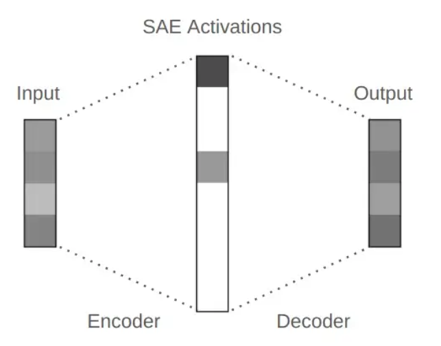
Traditional AEs usually learn compressed representations through a lower-dimensional bottleneck, and VAEs add probabilistic constraints on top of that hidden layer. Modern SAEs work differently. They usually use an overcomplete latent space, meaning the hidden layer is much larger than the input activation dimension. So the middle stage is not a compression step at all. It is an expansion step, giving the model an overcomplete dictionary in which it can represent latent features that greatly outnumber the original dimensions.
Ultralytics gives a clearer explanation: unlike standard compression methods that reduce dimensionality, SAEs usually use an “overcomplete” hidden layer, meaning the hidden layer has more neurons than the input layer. This creates a large feature dictionary, while the sparsity constraint ensures that only a small number of those features are used to describe any particular input.
Feature decoupling: in complex models, a single neuron often encodes multiple unrelated concepts, a phenomenon referred to here as superposition. SAE helps disentangle those concepts and assign them to different features.
For example, suppose we want to study layer 20 of a Transformer inside an LLM. We feed a large amount of text into the model after tokenization. If that layer has 4096 dimensions, then each token produces a 4096-dimensional activation vector. After running billions of tokens, we obtain a huge activation dataset, and that is what the SAE is trained to model and disentangle.
The SAE itself is a separate model. Its input is the activation vector produced by the LLM. The encoder expands that vector into, say, a 100k-dimensional latent space, and the decoder maps it back into the original activation space. The loss combines reconstruction loss with a sparsity penalty.
The complete data flow is: Raw Text -> Tokenizer -> Token IDs -> LLM -> Layer 20 activation -> SAE
Once the SAE is trained, you can run a large amount of text through both the LLM and the SAE, then record which tokens or contexts produce the strongest activations for each sparse feature. By looking at the shared semantic patterns in those high-activation samples, you can infer what that feature dimension might mean.
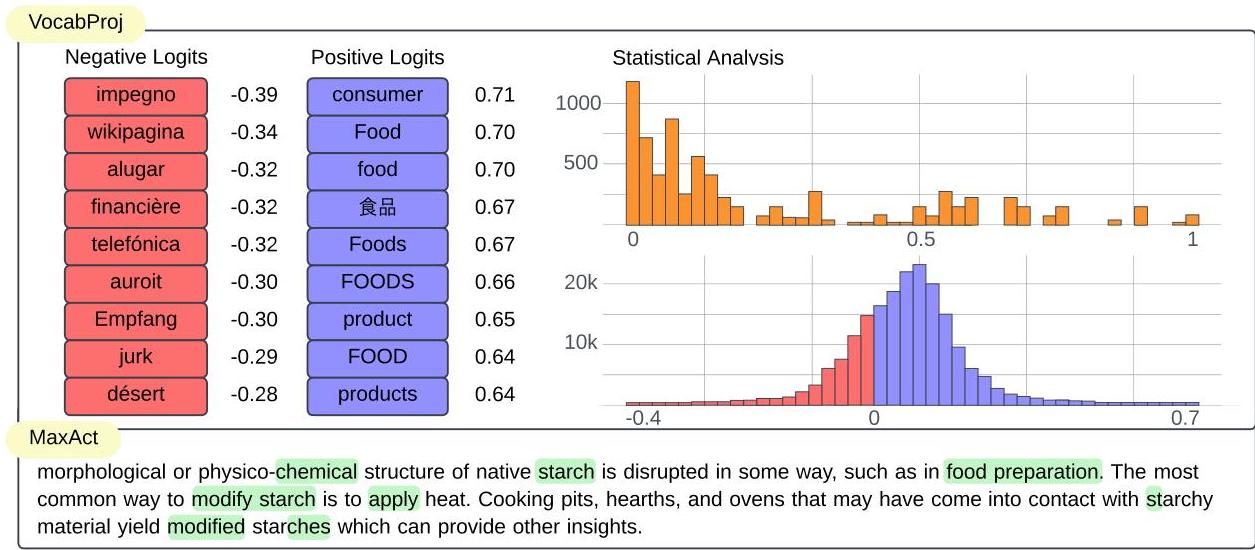
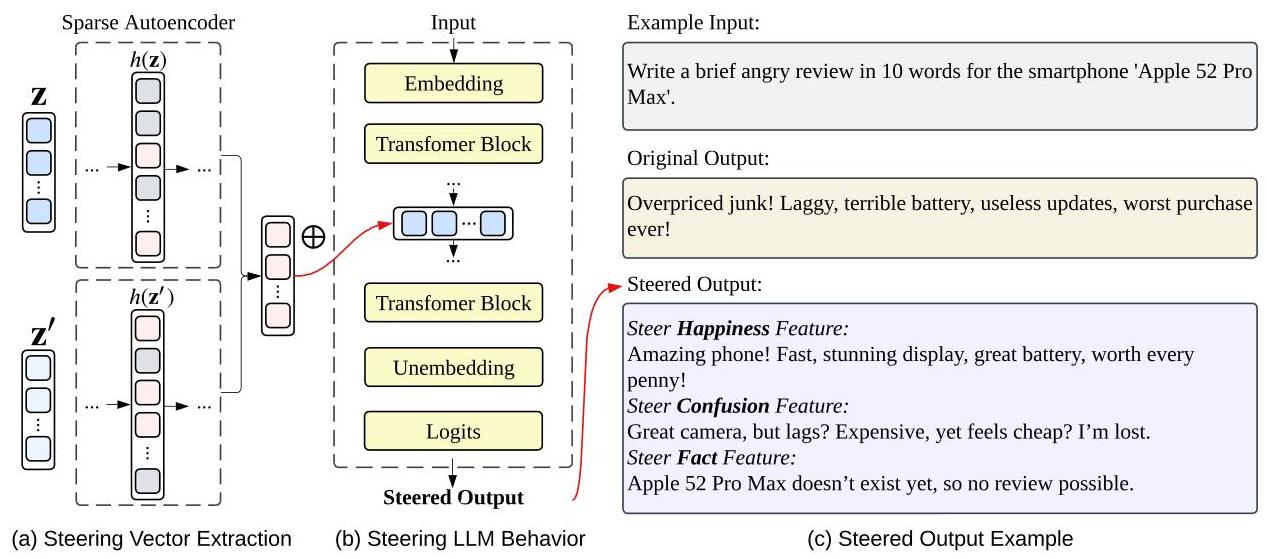
In a more concrete exploratory application, suppose a model often hallucinates citations to papers. You might discover that certain SAE features, say feature #1873, activate unusually strongly when the input contains fabricated author names or fabricated paper titles. That would let you form the hypothesis that feature #1873 is related to fake-paper hallucinations, and researchers could then selectively amplify or suppress that feature to steer the model’s responses.
Basic SAE Implementation
Here is a minimal SAE implementation. At its core, it is simply a network that expands the representation and then projects it back down.
import torch
import torch.nn as nn
import torch.nn.functional as F


class SparseAutoencoder(nn.Module):
    def __init__(self, input_dim, hidden_dim):
        super().__init__()
        # encoder
        self.encoder = nn.Linear(input_dim, hidden_dim)
        # decoder
        self.decoder = nn.Linear(hidden_dim, input_dim)

    def forward(self, x):
        # activation
        latent = F.relu(self.encoder(x))
        # decoder reconstruction
        reconstruction = self.decoder(latent)
        return reconstruction, latent


# Example usage
model = SparseAutoencoder(input_dim=784, hidden_dim=1024)
dummy_input = torch.randn(1, 784)
recon, latent_acts = model(dummy_input)

# During training, add the mean absolute value of activations and l1 regularization to loss
# loss = reconstruction_loss + lambda * torch.mean(torch.abs(latent_acts))
print(f"Latent representation shape: {latent_acts.shape}")
2026/8/12 in Suzhou