Decision trees are fundamental models. Over time, researchers extended them into ensemble learning, giving us the familiar Bagging and Boosting families. Bagging aggregates the votes or averages of many decision trees to form a random forest. Boosting trains trees sequentially, with each new tree focusing on the residual left by all preceding trees, then outputs a weighted sum.

Bagging and random forests

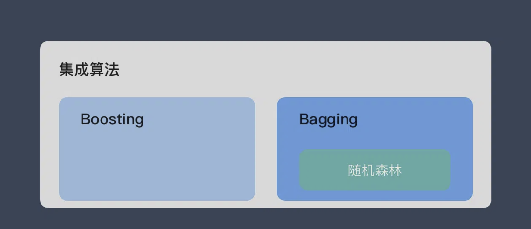
Random forests improve performance by combining multiple trees. A single tree easily overfits because its variance is large, so multiple trees are needed to balance it. This also means subtrees must not be too similar: covariance between trees should be low.

$$\mathrm{Var}(\hat{f}) = \frac{1}{T} \mathrm{Var}(\text{single tree}) + \left(1 - \frac{1}{T}\right) \mathrm{Cov}(\text{tree}_i, \text{tree}_j).$$

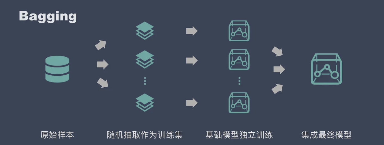
Random forests reduce correlation across trees through data randomness and feature randomness: bootstrap sampling for the former, random feature selection for the latter.

Bootstrap sampling

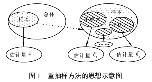
Bootstrap is an early resampling technique. It repeatedly draws subsamples with replacement to simulate the population distribution and estimate it. It does not require a particular distribution, unlike t-tests and z-tests, which assume normality.

Repeated sampling also works for small datasets because the generated virtual sample volume can estimate the distribution. Repetition weakens the impact of outliers and noise.

Random feature selection

At each split, a random forest does not consider all features. It selects a subset at random, allowing weaker features to remain available rather than being repeatedly excluded. Different nodes in one tree can focus on different feature combinations: one might use age and income, while the next uses gender and occupation.

Using only a subset is important because experiments show that using all features at every split reduces accuracy. If the subset is too small—only one feature—individual trees become weak and bias rises. If it is too large, every subtree becomes an ordinary decision tree, defeating Bagging’s purpose and raising variance.

Industrial implementation

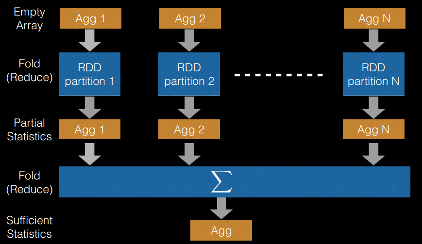
Random forests have the advantage that their trees can be trained in parallel, which made them popular early in industry. Distributed use still needs significant optimization, mainly in data storage and feature splitting. Spark MLlib stores data in RDDs and partitions; cluster workers independently obtain random data and train trees, then independently find optimal feature split points.

The following implementation notes are excerpted from GitHub:

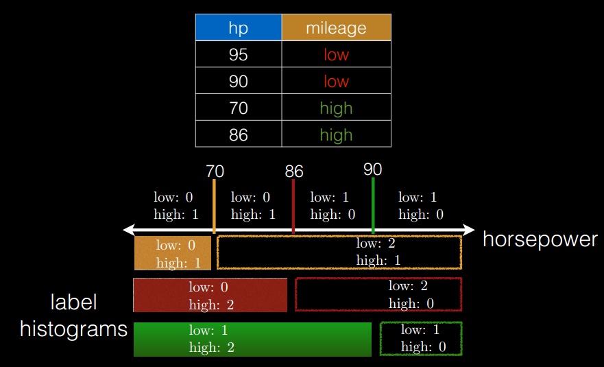
• Split-point sampling. On one machine, continuous-feature split points can be found by sorting values and taking points between adjacent values. At distributed or PB scale, that would cause excessive network transfer. Spark samples subfeatures in each partition, produces partition statistics, and derives split points from them.

• Feature binning. Tree construction repeatedly partitions feature values. A discrete feature with $M$ unordered values has up to $2^{M-1}-1$ partitions; if values are ordered, it has at most $M-1$. Three unordered age groups—old, middle, young—have three partitions; ordered groups have only two. Continuous features partition ranges at split points into bins. Because a distributed system cannot enumerate all continuous values, Spark uses sampled split-point statistics.

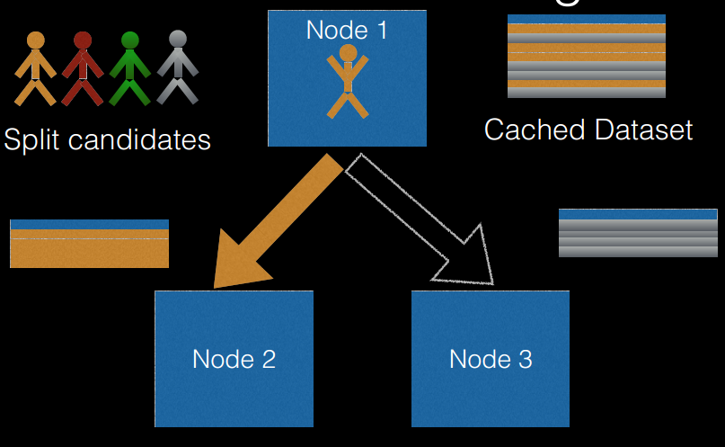
• Level-wise training. A single-machine tree is built recursively, essentially depth first, moving each child node’s data together. That is inefficient and often impossible for distributed datasets. A distributed tree is built level by level, essentially breadth first. The number of full data scans equals the maximum depth across trees. On every scan, the system calculates split statistics for all nodes, then decides whether and how to split them.

Boosting and AdaBoost

Boosting trains a new learner to fit the current ensemble’s residual, gradually reducing error. It comes from the idea of strong and weak learnability: an algorithm that learns a prediction class with high accuracy is strongly learnable, while one that is only slightly better than random guessing is weakly learnable. The two were later shown to be theoretically equivalent, meaning weak learners can be boosted into a strong learner.

Weak algorithms are simpler than directly learning a strong one, so boosting combines many weak learners. AdaBoost is an early example.

AdaBoost

AdaBoost also uses sample weights to distinguish hard and easy samples. In the first round, every example has equal weight. For $N$ samples:

$$w_i^{(1)} = \frac{1}{N} \quad (i = 1, 2, \dots, N).$$

Train the first weak classifier and calculate its weighted error rate. That error determines the classifier weight: lower error yields higher weight.

$$\alpha_t = \frac{1}{2} \ln\left( \frac{1 - \epsilon_t}{\epsilon_t} \right).$$

After the first classifier, update sample weights. Incorrect examples receive greater weight:

$$w_i^{(t+1)} = \frac{w_i^{(t)} \cdot e^{-\alpha_t y_i h_t(x_i)}}{Z_t},$$

where $Z_t$ normalizes the weights to sum to 1. Train the next weak classifier and update sample and classifier weights in the same way. The final prediction is a weighted vote of all weak classifiers.

Advantages:

• Cascades weak classifiers.
• Can use different algorithms as weak learners.
• Explicitly considers every classifier’s weight, unlike Bagging.

Disadvantages:

• The number of iterations, or weak learners, is difficult to choose.
• Class imbalance can reduce classification accuracy.
• Training is costly because the best split must be chosen again for every classifier.

March 16, 2025, Suzhou