understanding AUC in depth

Original article: Understanding AUC in Depth

AUC is one of the most common and widely used machine-learning evaluation metrics. Although its definition is geometric, its interpretation and applications are important. This post summarizes the original article.

• What is AUC?
• A probabilistic interpretation
  • Proof
  • AUC as a ranking metric
  • Insensitivity to class proportions
• Computing AUC
• Optimizing AUC
• What AUC makes a model good?

What is AUC?

In statistics and machine learning, AUC is commonly used to evaluate binary classifiers. It stands for area under the curve, where the curve is usually the receiver operating characteristic (ROC). Unlike threshold-dependent metrics such as accuracy, recall, and F1, AUC does not depend on a chosen classification threshold.

ROC curves were used in electronic and radar engineering during World War II for military target detection. They were later adopted in psychology, medicine, machine learning, and data mining.

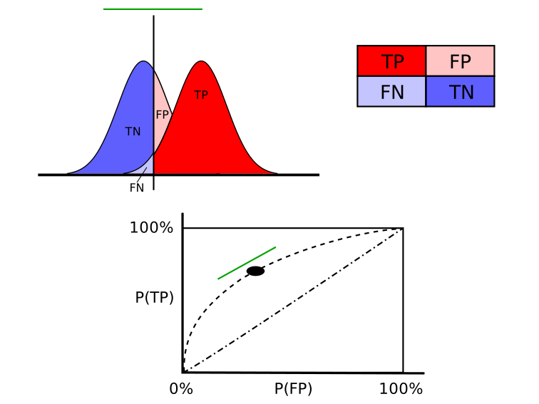
For a binary classification problem, a model predicts a score $s$ or probability $p$ for every sample. Given a threshold $t$, samples with $s > t$ are predicted positive and those with $s < t$ negative. This yields four outcomes:

	Actual positive	Actual negative
Predicted positive	TP (true positive)	FP (false positive)
Predicted negative	FN (false negative)	TN (true negative)

Different thresholds produce different proportions of these four cases. The true-positive rate (TPR) and false-positive rate (FPR) are defined as:

$$\text{TPR} = \frac{\text{TP}}{\text{TP} + \text{FN}}$$ $$\text{FPR} = \frac{\text{FP}}{\text{FP} + \text{TN}}$$

Let $N_+(t)$ and $N_-(t)$ be the numbers of positive and negative samples whose scores exceed $t$, and let $N_+$ and $N_-$ be the total counts. Then:

$$\text{TPR}(t) = \frac{N_+(t)}{N_+}, \qquad \text{FPR}(t) = \frac{N_-(t)}{N_-}.$$

As $t$ changes, TPR and FPR trace the ROC curve. A random model has no ability to distinguish classes, so the class ratio above the threshold is roughly the overall class ratio:

$$\frac{N_+(t)}{N_-(t)} = \frac{N_+}{N_-}.$$

Therefore TPR equals FPR, and the ROC curve is a straight diagonal. At the other extreme, a perfect model gives every positive sample a higher score than every negative sample, producing an L-shaped ROC curve. Real models lie between these cases, generally with a concave ROC curve. The area beneath it is AUC:

$$AUC = \int_{t = \infty}^{-\infty} y(t)\,d x(t),$$

where $x$ and $y$ are FPR and TPR, the horizontal and vertical axes of the ROC curve.

A probabilistic interpretation

Proof

AUC is widely used to measure ranking quality because it equals the probability that a randomly selected positive sample receives a higher score than a randomly selected negative sample. Consider the probability that the negative sample’s score lies in $[t, t + \Delta t]$:

$$P(t \leq s_{-} < t + \Delta t) = P(s_{-} > t) - P(s_{-}> t + \Delta t) = \frac{N_{-}(t) - N_{-}(t + \Delta t)}{N_{-}} = x(t) - x(t + \Delta t) = -\Delta x(t).$$

When $\Delta t$ is small, the conditional probability that the positive score exceeds the negative score is approximately:

$$P(s_+ > s_- \mid t \leq s_- < t + \Delta t) \approx P(s_+ > t) = \frac{N_+(t)}{N_+} = y(t).$$

Thus:

$$P(s_+ > s_-) = \sum P(t \leq s_- < t + \Delta t)P(s_+ > s_- \mid t \leq s_- < t + \Delta t) = -\sum y(t)\Delta x(t) = -\int_{t=-\infty}^{\infty} y(t)dx(t) = \int_{t=\infty}^{-\infty} y(t)dx(t).$$

The integration bounds matter: $t=-\infty$ corresponds to the top-right ROC point, while $t=\infty$ corresponds to the bottom-left point. Each infinitesimal term represents the event that a random negative has score $t$ and a random positive scores higher. Integrating yields the desired probability.

AUC as a ranking metric

The interpretation above says exactly that AUC is the probability of ranking a positive above a negative, which makes it useful for ranking models in search and recommendation. Adding a constant to every sample score does not change that probability, so it does not change AUC. In advertising scenarios that require well-calibrated absolute click-through probabilities, AUC is therefore not sufficient; metrics such as log loss are more appropriate.

Insensitivity to class proportions

The same interpretation shows that AUC is insensitive to the positive-to-negative ratio. With extreme imbalance, such as 1:1000, negative examples are commonly downsampled for training. If that sampling is random, AUC computed on the downsampled test set is essentially unchanged from AUC on the original set. For a positive example with score $s_+$, the share of negatives scoring below $s_+$ is unchanged by uniform sampling.

By contrast, downsampling negatives can overestimate accuracy because real negatives are removed; recall is unaffected because positives are retained. Together, this can overestimate F1.

Computing AUC

AUC can be computed directly from the ROC curve with trapezoidal integration. It can also be calculated through its relationship to the Wilcoxon–Mann–Whitney U statistic.

Sort positive and negative test samples by predicted score in ascending order. For the $j$th positive sample with rank $r_j$, there are $r_j - 1$ samples before it, of which $j - 1$ are positive. Therefore $r_j - j$ negatives have lower scores. Averaging the probability over all positives gives:

$$\frac{1}{N_+} \sum_{j=1}^{N_+} \frac{r_j - j}{N_-} = \frac{\sum_{j=1}^{N_+} r_j - \frac{N_+(N_+ + 1)}{2}}{N_+N_-}.$$

Hence:

$$\text{AUC} = \frac{\sum_{j=1}^{N_+} r_j - \dfrac{N_+(N_+ + 1)}{2}}{N_+ N_-}.$$

The corresponding SQL is:

select
    (ry - 0.5*n1*(n1+1))/n0/n1 as auc
from(
    select
        sum(if(y=0, 1, 0)) as n0,
        sum(if(y=1, 1, 0)) as n1,
        sum(if(y=1, r, 0)) as ry
    from(
        select y, row_number() over(order by score asc) as r
        from(
            select y, score
            from some.table
        )A
    )B
)C

Optimizing AUC

Maximum likelihood estimation corresponds to log loss, not AUC. In ranking problems, AUC may align more closely with the actual objective, so optimizing it directly can outperform maximum likelihood. Pairwise objectives can be viewed as AUC approximations because they act on score differences between positive and negative examples.

Method	Loss function
RankSVM	max(0, -s₊ + s₋ + Δ)
RankNet	log(1 + exp(-(s₊ - s₋)))
Exponential loss	exp(-(s₊ - s₋))
TOP loss	∑ₛ₊ max(0, -s₊ + s₋ + Δ)

These losses penalize positive-negative pairs for which $s_+ < s_-$. A closer AUC approximation is:

$$E \left[ (1 - w^T(s_+ - s_-))^2 \right] = \frac{1}{n_+ n_-} \sum_{i=1}^{n_+} \sum_{j=1}^{n_-} (1 - w^T(s_i^+ - s_j^-))^2.$$

Here $s_i^+$ and $s_i^-$ are positive and negative scores. This explains why ranking losses can outperform log loss when ranking matters more than probability calibration.

What AUC makes a model good?

Higher AUC means stronger separation between positive and negative examples, but there is no universal good threshold. In practice, click-prediction models often have substantially lower AUC than purchase-prediction models; purchase prediction among monthly active users and daily active users can also differ substantially, as can prediction over the next hour versus the next day. AUC is highly task-dependent.

Purchases usually carry a higher decision cost than clicks. Click behavior is more casual and harder to predict, so click-through-rate models commonly have lower AUC than purchase-rate models. Monthly active users are generally easier to separate into purchasers and non-purchasers than daily active users because the former include many recently inactive users, giving the monthly model a higher AUC.

Longer prediction horizons are also harder: more unexpected events can happen. Predicting what someone will do in the next second can simply predict their current action, whereas long-term behavior is much harder to foresee. A one-day purchase model will therefore generally have a lower AUC than a one-hour model.

June 22, 2025, Suzhou