References:

Understanding node2vec Node2vec in WeChat Moments lookalike algorithms Complete guide to understanding Node2Vec

Earlier post: Word2Vec in PyTorch

Node2Vec follows an intuition: random walks in a graph can be treated like sentences in a corpus. Every graph node is a word, and every random walk is a sentence.

At work, I encountered a nested feature made of sequential events. One sample can contain multiple events of unequal length; every event has a structured format and a category.

The earlier approach was to calculate time-window statistics for fixed categories. With $n$ event categories and $d$ time windows, this creates $n \times d$ extra features, such as the number of A events in the last three days or B events in the last five days.

Sequences have unequal length and can introduce unknown event types over time. If a new inference set contains unknown event C, the feature cannot be handled directly. It could be combined into a single unknown category, but that distorts the distribution of different event types.

There are also dimensionality and sparsity problems. Ten event categories over 3-, 5-, and 7-day windows create 30 features; 20 categories create 60. Because of the task’s nature, most are zero. Rapidly growing sparse features require an enormous dataset to fit.

Could we embed them instead? Every sample has a variable-length array that represents both temporal order and preferences over categories. When manually processing categories forward is difficult, we can reverse the perspective and build graph features from how often categories connect to samples.

Graph embeddings have a long history. Node2Vec is one embedding algorithm that followed Word2Vec.

Node2Vec and Word2Vec

Node2Vec and Word2Vec share the goal of learning co-occurrence relationships between items from constructed sequences. Word2Vec uses a sliding window to form target-context word pairs, then one-hot encodes every vocabulary word.

For Skip-Gram, take “the weather is great today” as a corpus, tokenized into three words: today, weather, and great; vocabulary size is $V=3$, embedding dimension $d=4$. We want to predict the two surrounding words given weather. With window size 1, the pairs are today → weather, weather → today, weather → great, and great → weather.

weather has index 1 and one-hot vector $x_{\text{weather}} = [0, 1, 0]$. An embedding matrix $W$ of size $V \times d = 3 \times 4$ maps it to a low-dimensional vector $h = W^T \cdot x$.

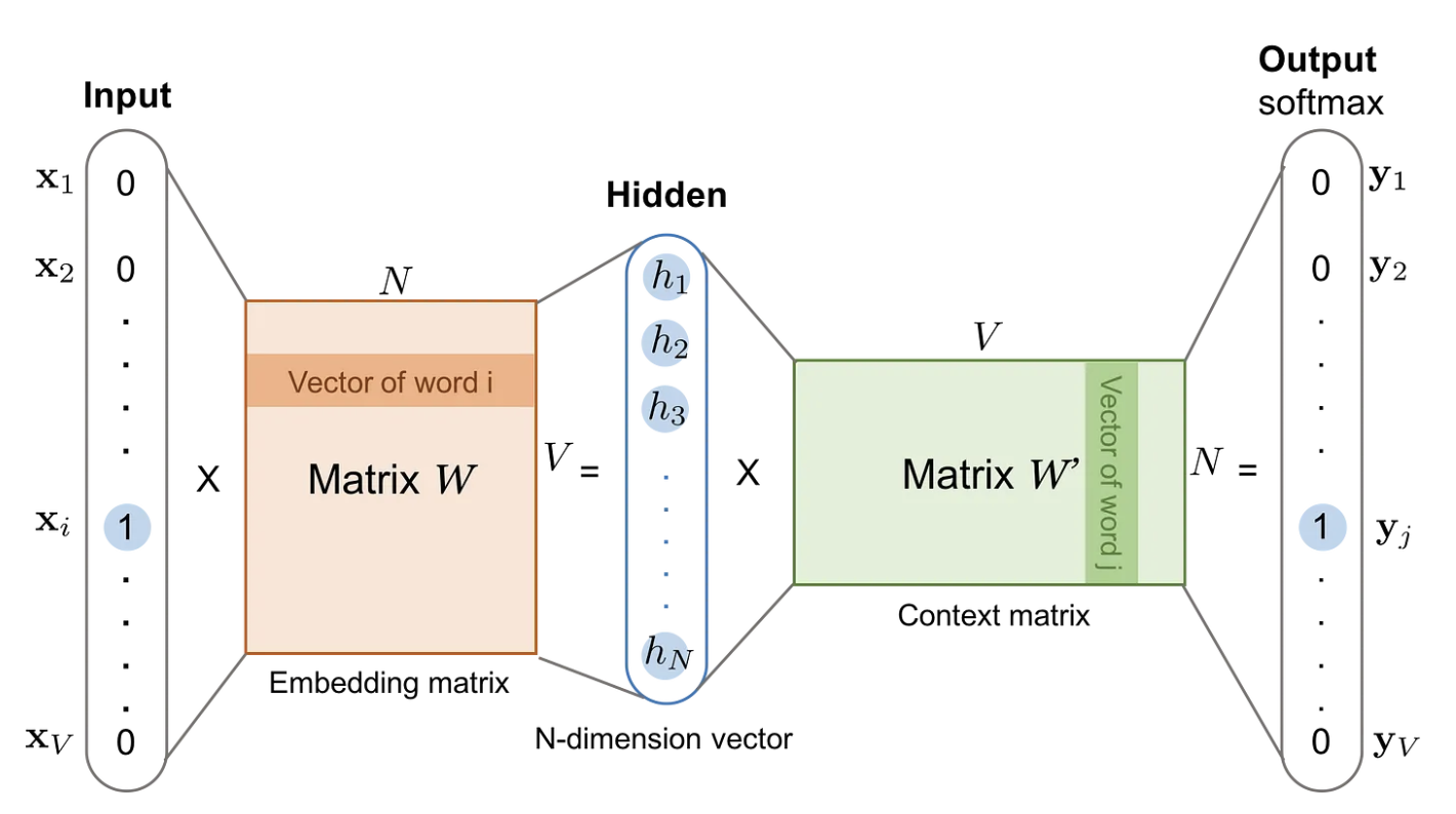
Dimension changes:

• Input $x$: $V = 3$.
• Embedding matrix $W$: $(V, d) = (3, 4)$.
• Output $h$: $d = 4$.

At the output layer, another $d \times V$ matrix $W'$ produces predicted probabilities normalized by Softmax. Cross-entropy loss and backpropagation train the embedding matrix. Multiplying a one-hot word vector by that matrix selects its $1 \times d$ embedding row, which is why embeddings are fundamentally lookup tables.

Word2Vec obtains sequences from contextual windows. DeepWalk applied the same idea to graphs in 2014: starting from a node, randomly sample successive nodes, then train Skip-Gram on the resulting sequences. Node2Vec made a small but important improvement two years later.

Random walks

Graph embedding mostly revolves around sequence construction, and random walks are a key innovation. In a graph, a random walk starts from one node and visits neighbors under a probability rule. Consider:

    A -- B -- C
     \       /
      D --- E

Starting at A and choosing neighbors with equal probability could produce:

A → B → C → E → D → A → D → E → C

This is a random-walk path. In an unweighted graph, each neighbor is selected equally; in a weighted graph, selection follows edge weights. A biased random walk can instead prefer depth-first-search-like or breadth-first-search-like behavior. The former visits more distant nodes, while the latter prioritizes nearby nodes.

Node2Vec introduces two parameters for biased walks:

• Return parameter $p$ controls whether the walk returns to the previous node. Larger $p$ makes returning less likely.
• In-out parameter $q$ balances BFS and DFS. $q > 1$ favors BFS, or local exploration; $q < 1$ favors DFS, or deeper exploration.

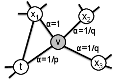
The transition probability is $\pi_{vx} = \alpha(t, x) \cdot w_{vx}$, where $w_{vx}$ is the edge weight between $(v, x)$—usually 1 for an unweighted graph—and $\alpha(t, x)$ controls the preference from previous node $t$ to new node $x$.

A first-order random walk considers only the next-node probability. Node2Vec uses a second-order relationship and therefore needs two parameters to refer back to the previous node.

Challenges in industrial implementations

Three difficulties became clear while writing code:

1. Graph algorithms often run out of memory. At tens of millions of nodes, neighboring nodes and edges can number in the millions or tens of millions, requiring hundreds of gigabytes.
2. It remains unclear how to combine statistical features with embeddings. Earlier industrial recommendation systems modeled statistics and embeddings separately, as in Wide & Deep, and merged the results. Later approaches concatenate them directly, but there is no generally accepted effective approach.
3. How should edge weights be calculated, and how should cold-start users be handled?

Related Zhihu discussion: How can deep learning incorporate statistical features?

March 1, 2025, Suzhou